The way it functions (Part 3)

In this article, we are going to scrutinize both surjective (onto) and injective (one-to-one) functions and study their significance. Recall that we first introduced them in Remark 9.1 in a more or less informal setting. Here, we are going to first rephrase their definitions using the function notation that was brought to the table in Part 2, and then deepen our understanding with the aid of examples.

Surjective (Onto) functions

Definition

Let f be a function mapping from A to B

$\displaystyle f:A\longrightarrow B$

We say that f is surjective if for every element y in B there exists some element x in A such that f(x) = y.

Discussion

As an aside, in mathematics, we use the determiner “some” to mean “at least one”, i.e. we don’t rule out the possibility that two or more elements possess the said property.

Now let’s try to discern the definition. All it’s really saying is that there is no redundancy in the codomain B: every element of the codomain B is a target of some source in domain A, and so every element of the codomain is a valid output of the function f.

In the context of algebra, a function f is surjective if for every y in the codomain B, the equation

$\displaystyle f(x)=y$

always has a solution x in the domain A.

To illustrate this idea, consider the function

$\displaystyle f:\mathbb{R}\longrightarrow \left[0, +\infty\right)$

$\displaystyle f(x) = x^2$

whose domain is the set of all real numbers, and codomain the set of all non-negative real numbers. We claim that f is surjective, but how do we verify that? Well, it amounts to solving the equation

$\displaystyle x^2=y$

for any non-negative real number y. Since x is a real number, we can simply set $\displaystyle x=\sqrt{y}$ so that

$\displaystyle x^2=\left(\sqrt{y}\right)^2=y$

For instance, if y = 4, we can set x = 2 so that

$\displaystyle f(2)=2^2=4$

Similarly, if y = 5, we can set $\displaystyle x=\sqrt{5}$ so that

$\displaystyle f\left(\sqrt{5}\right)=\left(\sqrt{5}\right)^2=5$

In contrast, let’s look at the function

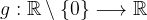
$\displaystyle g:\mathbb{R}\setminus \{0\} \longrightarrow \mathbb{R}$

$\displaystyle g(x) = \frac{1}{x}$

whose domain is the set of all non-zero real numbers and codomain the set of all real numbers. Function g is not surjective because 0 is an element of the codomain, but it’s not a valid output of g. In other words, the equation

$\displaystyle \frac{1}{x}=0$

has no real number solution x.

To summarize, tracing the source (or sources) of every element of the codomain is made possible by the surjective property of the function.

Injective (One-to-one) functions

Definition

Let g be a function mapping from A to B

$\displaystyle g:A\longrightarrow B$

We say that g is injective whenever g(x₁) = g(x₂) in B implies x₁ = x₂ in A.

Discussion

A logically equivalent condition for injectivity would be “whenever x₁ ≠ x₂ in A implies g(x₁) ≠ g(x₂) in B”.

Essentially, no two different sources share the same target in the codomain. One implication is that we can identify every element in the image set g(A) (see Remark 10.1) with exactly one element in the domain A, and in this sense, the domain A lives in the codomain B as the image set g(A).

Perhaps the greatest significance of the injective property is this: starting from the image set, we are able to travel backward to the domain, and the reverse relationship is itself a function (more on this in future post).

Algebraically speaking, a function g is injective if for every output y in the image g(A), the equation

$\displaystyle g(x)=y$

has only one solution x in the domain A.

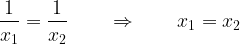
Let’s recycle the previous two example functions to demonstrate this notion. Firstly, the function

$\displaystyle g:\mathbb{R}\setminus \{0\} \longrightarrow \mathbb{R}$

$\displaystyle g(x) = \frac{1}{x}$

is injective because given any nonzero number y (recall that 0 is not a valid output), the equation

$\displaystyle \frac{1}{x}=y$

has a unique solution x = 1/y. Equivalently,

$\displaystyle \frac{1}{x_1}=\frac{1}{x_2}\qquad\Rightarrow\qquad x_1=x_2$

Next, the function

$\displaystyle f:\mathbb{R}\longrightarrow \left[0, +\infty\right)$

$\displaystyle f(x) = x^2$

is not injective since for a positive number y, the equation

$\displaystyle x^2=y$

has two distinct solutions

$\displaystyle x=\sqrt{y}\qquad\text{or}\qquad x=-\sqrt{y}$

Simply put, the injective property is the key to reversing the roles of inputs and outputs unambiguously: every output points to one and only one input.

More (real life) examples

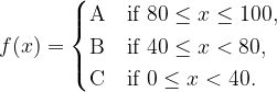
Let’s suppose there was a group of four students who sat for an exam that was scored out of 100 points. The score would subsequently be converted into a grade. This grading process can be regarded as a function f from the set of possible scores to the set of all possible grades.

$\displaystyle P=\left\{\text{all possible scores from 0 to 100 points} \right\}\\\\Q=\left\{\text{A, B, C} \right\}$

$\displaystyle f:P\longrightarrow Q$

$\displaystyle f(x)=\begin{cases} \text{A} & \text{if }80\leq x \leq 100, \\ \text{B} & \text{if } 40\leq x < 80, \\ \text{C} & \text{if } 0\leq x < 40. \end{cases}$

On the other hand, each of the exam candidates was given a unique 3-digit ID number upon registration. This assignment can also be seen as a function g from the set of all candidates to the set of all possible 3-digit ID.

$\displaystyle R=\left\{\text{Felix, Jenna, Sheba, Piers} \right\}\\\\S=\left\{\text{all 3-digit ID numbers} \right\}$

$\displaystyle g:R\longrightarrow S$

$\begin{aligned} &g(\text{Felix}) &= 001\\&g(\text{Jenna}) &= 002\\&g(\text{Sheba}) &= 003\\&g(\text{Piers}) &= 004\end{aligned}$

When the exam result was ready, a report card that shows the ID number and the grade was generated for each student. A bare bone example is shown below.

Now it’s time to analyse the two functions. First, it’s obvious that f is surjective, which means that we can meaningfully interpret any grades from A to C and trace the range of scores. However, the fact that f is not injective means that it is impossible to pinpoint the exact score behind the given grade. For instance, we know from the report card that the student with ID 001 was awarded an A grade, which can be interpreted as the highest grade according to function f. But we cannot know how excellent 001 performed score-wise since any score between 80 and 100 points yields the same grade.

Moving on to function g, we see that it is injective. Hence, given any of the four assigned ID numbers (i.e. valid outputs), we can tell exactly who the student is. Looking at the report card again, we can say for sure that it’s Felix who obtained an A grade in this exam since ID 001 is uniquely paired with Felix. On the other hand, g is clearly not surjective, and so we cannot meaningfully interpret ID numbers like 005 or 032 as they don’t point to any exam candidates.

Conclusion

The real-life scenario above showcases how versatile the concept of functions is. Indeed, the surjective grading function f is used to model a grouping process, whereas the injective ID number function g is an archetype of a renaming process. A natural question to ask next is what can we say about a function that is bijective (i.e. injective and surjective)? The answer is tied closely to the concept of inverse function, which we will explore in future. Until then, stay acute, stay safe. See you!

Remark 11.1

Let’s revisit the grading function f in the real-life scenario. At one point, we saw that f is not injective, and so we can never recover the original score from the grade. More generally, a many-to-one function causes a loss of information. This may sound bad at first, but from another perspective, a many-to-one function also helps in the reduction of noise.

So what really matters is how much we value the inputs of the function, and that will in turn determine how we want to “group” them. This of course depends on the situation. To demonstrate, suppose we want to differentiate between the students’ performances even more. We can come up with a finer grading system f₁ as follows:

$\displaystyle P=\left\{\text{all possible scores from 0 to 100 points} \right\}\\\\Q_1=\left\{\text{A+, A, B+, B, C+, C} \right\}$

$\displaystyle f_1:P\longrightarrow Q_1$

$\displaystyle f_1(x)=\begin{cases} \text{A+} & \text{if }90\leq x \leq 100, \\ \text{A} & \text{if } 80\leq x < 90, \\ \text{B+} & \text{if } 60\leq x < 80, \\ \text{B} & \text{if } 40\leq x < 60, \\ \text{C+} & \text{if } 20\leq x < 40, \\ \text{C} & \text{if } 0\leq x < 20. \end{cases}$

Conversely, if all we care about is whether students pass or fail the exam, we can just use a coarser grading system f₂ as follows:

$\displaystyle P=\left\{\text{all possible scores from 0 to 100 points} \right\}\\\\Q_2=\left\{\text{Pass, Fail} \right\}$

$\displaystyle f_2:P\longrightarrow Q_2$

$\displaystyle f_2(x)=\begin{cases} \text{Pass} & \text{if }40\leq x \leq 100, \\ \text{Fail} & \text{if } 0\leq x < 40. \end{cases}$

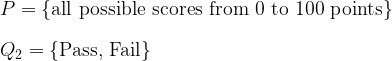
In conclusion, to construct the range (or codomain) of our function, we ought to decide whether certain aspects of the inputs should be perceived as information or noise – they are just two sides of the same coin.

Surjective (Onto) functions

Definition

Discussion

Injective (One-to-one) functions

Definition

Discussion

More (real life) examples

Conclusion

Remark 11.1

You Might Also Like

This Post Has One Comment