Raters gonna rate - Acute Angel

We live in a world that is extraordinarily dynamic. Understanding the world is therefore in large part about understanding how things change. Enter the concept of rate, which is far from being a foreign idea, really. Indeed, you measure the speed of a moving object as a rate of change of its position. Your heart rate is one of the many indicators of your physical health. You heat the kettle to speed up the reaction rate of vaporization of water so that it boils. Undoubtedly, the idea of rate is relevant to many aspects of our daily life.

That said, the notion of rate is quite a tricky concept to grasp. Firstly, it naturally involves division and fraction, both of which are usually the stumbling blocks for those who’ve just started learning elementary level math. Often times, many young learners find it hard to wrap their heads around the concept of rate as they also struggle with division and fraction.

Secondly, and more crucially, many rates in real life do not stay constant, and so they themselves are changing. In other words, they could be functions of some variables (see Remark 12.1), and that of course adds an extra layer of complexity to the analysis.

For the purpose of this article, we will take a modest step and focus on just the simple case of constant rate. Even then, there are already some subtleties that require careful treatment, as we shall see.

Constant rate as a ratio and fraction

A rate is a special kind of ratio that relates two or more quantities that are usually in different units. As an illustration, consider a train moving at a constant speed of 200 km per hour. Let’s dissect the phrase “constant speed of 200 km per hour”.

Here, the train speed is a ratio that relates the distance travelled by the train, in kilometres, to the time interval, in hours. The speed being constant means that the ratio is fixed, regardless of where the train is at or how much time has elapsed. Finally, the phrase “200 km per hour” means that for every 1 hour of duration of travel, a distance of 200 km is covered by the train.

The train travels 200 km in every 1-hour interval.

Being a ratio of some sort, a rate can also be expressed as a fraction. Using the same train example, we can express the train speed as

$\displaystyle \text{speed} = \dfrac{200\;\text{km}}{1 \;\text{hour}}$

The fractional expression is especially versatile computationally as it inherits not only the form but also the arithmetic of fractions, and we will now investigate one instance how it can be useful.

Unit conversion and dimensional analysis

Humans have been taking all sorts of measurements since the dawn of civilization. As a result, a huge number of units of measurements have accrued, and it is therefore important to know how to convert from one to the other.

Expressing a rate as a fraction allows us to convert the units systematically via a process that mirrors the cancellation of common factor in fraction arithmetic. Let’s go through several examples to demonstrate the idea.

Example 12.1

Suppose an ant is crawling in a straight line at a constant rate of 6 inches per minute. How can we express the same speed in a different unit, say inches per second?

We know that 1 minute = 60 seconds, but let’s try to rewrite this equality in a rather strange way as follows:

$\displaystyle \dfrac{1 \;\text{minute}}{60 \;\text{second}}=1$

The fraction on the left is called a conversion factor, which is equivalent to 1. Consequently, multiplying the rate by a conversion factor only changes its form, and not its inherent value.

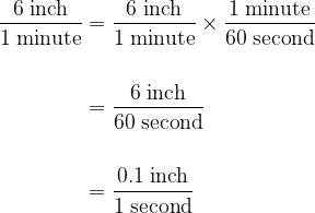
$\displaystyle \begin{aligned} \dfrac{6 \;\text{inch}}{1 \;\text{minute}} &=\dfrac{6 \;\text{inch}}{1 \;\text{minute}} \times \dfrac{1 \;\text{minute}}{60 \;\text{second}}\\\\&=\dfrac{6 \;\text{inch}}{60 \;\text{second}}\\\\&=\dfrac{0.1 \;\text{inch}}{1\;\text{second}}\end{aligned}$

Notice how we cancel the unit “minute” in the numerator and denominator so that the remaining units are exactly what we are after? This procedure of treating units in the same way we treat factors in fraction is called dimensional analysis, and it is widely used in the fields of science and engineering.

Example 12.2

What really makes dimensional analysis so powerful is that we can connect a series of carefully chosen conversion factors to obtain the desired units. For instance, here is how we can convert the ant’s speed from inches per minute to cm per second in one go by combining two conversion factors:

$\displaystyle \begin{aligned} \dfrac{6 \;\text{inch}}{1 \;\text{minute}} &=\dfrac{6 \;\text{inch}}{1 \;\text{minute}}\times \dfrac{2.54 \;\text{cm}}{1 \;\text{inch}} \times \dfrac{1 \;\text{minute}}{60 \;\text{second}}\\\\&=\dfrac{6 \times 2.54 \;\text{cm}}{60 \;\text{second}}\\\\&=\dfrac{0.254 \;\text{cm}}{1 \;\text{second}}\end{aligned}$

So far, all the calculations seem pretty straightforward. In fact, one might even find the inclusion of conversion factors in the working unnecessary. Looking back to Example 12.1, isn’t

$\displaystyle \dfrac{6 \;\text{inch}}{1 \;\text{minute}}=\dfrac{6 \;\text{inch}}{60 \;\text{second}}$

simply due to the fact that 1 minute is equivalent to 60 seconds?

A closer look at the conversion factor

A more accurate interpretation of the conversion factor $\displaystyle \frac{1\;\text{minute}}{60\;\text{second}}$ in Example 12.1 is not “1 minute is equivalent to 60 seconds”, but “a change of 1 minute is equivalent to a change of 60 seconds”.

Wait a minute (or 60 seconds) – is there really a difference between the two statements? Numerically, no; conceptually, yes.

To understand why, let the number of minutes be denoted by the variable m, and the corresponding number of seconds by the variable s. The statement “1 minute is equivalent to 60 seconds” comes from the relationship

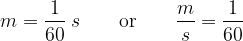
$\displaystyle m=\dfrac{1}{60}\: s\qquad \text{or}\qquad \dfrac{m}{s}=\dfrac{1}{60}$

On the other hand, using the customary notation to denote change, the statement “a change of 1 minute is equivalent to a change of 60 seconds” can be more generally written as

$\displaystyle \Delta m=\dfrac{1}{60}\,\Delta s\qquad \text{or}\qquad \dfrac{\Delta m}{\Delta s}=\dfrac{1}{60}$

From here we can see that, numerically,

$\displaystyle \dfrac{m}{s} =\dfrac{\Delta m}{\Delta s}$

even though both sides of the equality mean very different things conceptually. And in the context of unit conversion, the role of conversion factor is played by $\displaystyle \frac{\Delta m}{\Delta s}$ instead of $\displaystyle \frac{m}{s}$ .

Perhaps the next example is able to draw an even clearer distinction between the two types of ratio.

Example 12.3

A chemical solution with an initial temperature of 15 degrees Celsius (°C) is heated in a controlled setting so that its temperature rises at a constant rate of 1°C per minute. What is the rate of change of its temperature in degrees Fahrenheit (°F) per minute?

For people who are not familiar with the Fahrenheit scale (or the Celsius scale), to convert c degrees Celsius to f degrees Fahrenheit, we use the equation

$\displaystyle f =1.8c + 32$

Now, one might say, hey, since 1°C is equal to 33.8°F according to the equation above, can’t we just rewrite the rate as

$\displaystyle \dfrac{1\textdegree{}\text{C}}{1 \;\text{minute}} =\dfrac{33.8\textdegree{}\text{F}}{1 \;\text{minute}} \quad ?$

Well, we can check whether or not this makes sense by listing down several temperature values in both units at different times and then calculate the rate of change.

From the table, we see that every time we advance by 1 minute, the temperature of the solution increases only by 1.8°F, not 33.8°F! Hence, the statement “1°C is equivalent to 33.8°F” fails to convert the unit correctly.

Instead, what really matters is to know a change of 1 degree Celsius is equivalent to a change of how many degrees Fahrenheit. The clue is in the difference equation

$\displaystyle \Delta f =1.8\,\Delta c$

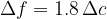
By letting $\displaystyle \Delta c = 1$ , we can solve for $\displaystyle \Delta f = 1.8$ . To spell it out, a change of 1°C is equivalent to a change of 1.8°F, and that means the conversion factor is $\displaystyle \frac{1.8\textdegree{}\text{F}}{1\textdegree{}\text{C}}$ so that

$\displaystyle \begin{aligned} \dfrac{1 \textdegree{}\text{C}}{1 \;\text{minute}} &=\dfrac{1 \textdegree{}\text{C}}{1 \;\text{minute}} \times \dfrac{1.8 \textdegree\text{F}}{1 \textdegree\text{C}}\\\\&=\dfrac{1.8 \textdegree{}\text{F}}{1 \;\text{minute}}\end{aligned}$

This time, the conversion agrees with what we observed in Table 12.1, so we know it is the right one.

Comparing Examples 12.1 and 12.3

Why, then, is there a numerical difference in Example 12.3, and why is such difference absent from Example 12.1 (where we convert minutes to seconds)? To answer this, let’s juxtapose the equations in Example 12.1 with those in Example 12.3 below.

$\displaystyle \begin{aligned} m=\dfrac{1}{60}\:s \qquad &\text{and}\qquad \Delta m=\dfrac{1}{60}\, \Delta s\\\\ f=1.8c + 32 \qquad &\text{and}\qquad \Delta f=1.8\,\Delta c \end{aligned}$

Also, it will be helpful if we equip ourselves with some math parlance. In general, we say that a variable y is directly proportional to a variable x when their ratio is a fixed number. In Example 12.1, m is directly proportional to s and $\displaystyle \Delta m$ is directly proportional to $\displaystyle \Delta s$ because

$\displaystyle \dfrac{m}{s} =\dfrac{1}{60}\qquad \text{and}\qquad \dfrac{\Delta m}{\Delta s}=\dfrac{1}{60}$

As we saw previously, both ratios are equal to the same number, so there is no numerical difference in using either of the two ratios.

This is not the case, however, in Example 12.3. In particular, f is not directly proportional to c. Indeed, the ratio

$\displaystyle \dfrac{f}{c} =1.8+\dfrac{32}{c}$

is not a constant as it depends on the value of c. On the other hand, $\displaystyle \Delta f$ is directly proportional to $\displaystyle \Delta c$ because

$\displaystyle \dfrac{\Delta f}{\Delta c}=1.8$

and it is this ratio that’s responsible for the unit conversion from °C per minute to °F per minute.

Now that we have addressed the difference, we should take note of one important similarity between the two examples: even though the original variables may or may not be directly proportional to each other, the changes of the variables are directly proportional to each other. This feature is tied closely to the concept of linearity, which is a topic for another time. Simply put, both m and f are linear functions of s and c, respectively.

We’ve now taken our first baby step to understanding the ever-changing world, though we will have to develop more tools before we can paint the full picture. So there’s more to learn, and that’s always good news. Until then, stay acute, stay positive. See you!

Remark 12.1

It was mentioned at the beginning of this post that many rates we encounter in real life are not fixed, and so they too change all the time. This means that in addition to the rate of change, we could also study the rate of change of the rate of change, and the rate of change of the rate of change of the rate of change, ad infinitum. This idea is related to the concept of higher order derivatives in calculus, which is, in essence, the study of change.

Remark 12.2

Back in Example 12.1, we wrote down this line of working in dimensional analysis:

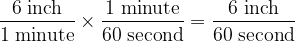
$\displaystyle \dfrac{6 \;\text{inch}}{1 \;\text{minute}} \times \dfrac{1 \;\text{minute}}{60 \;\text{second}} = \dfrac{6 \;\text{inch}}{60 \;\text{second}}$

For the sake of argument, let d denote the distance travelled by the ant, in inches. The above line of working can thus be reformulated algebraically as

$\displaystyle \dfrac{\Delta d}{\Delta m} \times \dfrac{\Delta m}{\Delta s} = \dfrac{\Delta d}{\Delta s}$

The above is just a special case of a formula in calculus called the chain rule that links different rates of change together, and it is of great theoretical and computational importance in mathematics.